
Plotting a stratigraphic column with rmacrostrat
Source:vignettes/stratigraphic-column.Rmd
stratigraphic-column.RmdAuthors: Palaeoverse Development Team
Last updated: 2025-05-06
Introduction
rmacrostrat is an R package which allows users to easily
retrieve geological data from the Macrostrat database and facilitates
analyses of these data within the R environment. This vignette (or
tutorial, if you prefer) is provided to guide you through the
installation process and some of the functionality available within
rmacrostrat. Specifically, we will focus on obtaining and
plotting a geologic column, containing stratigraphic and lithological
information for the San Juan Basin, located in the southwestern United
States.
Installation
The rmacrostrat package can be installed via CRAN, or
its dedicated GitHub repository
if the development version is preferred. To install via CRAN, simply
use:
install.packages("rmacrostrat")To install the development version, first install the
devtools package, and then use install_github
to install rmacrostrat directly from GitHub.
install.packages("devtools")
devtools::install_github("palaeoverse/rmacrostrat")
You can now load rmacrostrat using the default
library function, alongside some packages we will need for
plotting, namely ggplot2, ggrepel, and
deeptime (don’t forget to install these packages if you
don’t have them already!):
library(rmacrostrat)
# Install and load data visualization packages
library(ggplot2)
library(ggrepel)
library(deeptime)
Before we get into the good stuff, the development team has a
small request. If you use rmacrostrat in your
research, please cite the associated publication. This will help us to
continue our work in supporting you to do yours. You can access the
appropriate citation via:
citation("rmacrostrat")## To cite rmacrostrat in publications, use the following citation:
##
## Jones, L.A., Dean, C.D., Gearty, W., and Allen, B.J. 2024. rmacrostrat:
## An R package for accessing and retrieving data from the Macrostrat
## geological database. Geosphere, v. 20:6, 1456--1467. doi:
## 10.1130/GES02815.1
##
## A BibTeX entry for LaTeX users is
##
## @Article{,
## title = {rmacrostrat: An R Package for fetching geologic data from the Macrostrat database.},
## author = {Lewis A. Jones and Christopher D. Dean and William Gearty and Bethany J. Allen},
## year = {2024},
## journal = {Geosphere},
## volume = {20},
## number = {6},
## pages = {1456--1467},
## doi = {10.1130/GES02815.1},
## }Context
The San Juan Basin is a large structural depression which spans parts
of New Mexico, Colorado, Utah, and Arizona. It is renowned for its oil
and natural gas reserves, but it is also well-known for its late
Cretaceous dinosaurs. In this vignette, we will investigate the geologic
attributes of the rocks of the San Juan Basin and use this information
to plot a stratigraphic column. In order to do this, we will make use of
the rmacrostrat package to fetch data from the Macrostrat database.
Retrieving data
Our first step is to search for geologic columns named “San Juan
Basin” and retrieve some basic information about them, using the
def_columns function:
# Get column definitions for the San Juan Basin
def_columns(column_name = "San Juan Basin")
## col_id col_group_id col_name lat lng col_area max_thick ref_id
## 1 489 3 San Juan Basin 35.896 -108.068 35096.52 8040 1
## status t_units project_id notes
## 1 active 47 1 NAFrom this call, we can see there is a single column named “San Juan
Basin”. We are also given some information about this column, such as
its geographic location (in the form of a latitude and longitude), the
area over which it spans in km2, its thickness in meters, and
the number of geologic units it contains (t_units). We are
also given its col_id, 489, which we can use to retrieve
more information through other functions in rmacrostrat. We
will do this now, specifically using get_columns:
# Using the column ID, retrieve the San Juan Basin column
san_juan <- get_columns(column_id = 489)
Exploring data
We now have much more information relating to the San Juan Basin column. For example, we can look at the age range it spans:
# Print (numerical) age range of San Juan Basin column
san_juan$b_age
## [1] 2050
san_juan$t_age## [1] 32.38
# Print (interval) age range of the San Juan Basin column
san_juan$b_int_name
## [1] "Orosirian"
san_juan$t_int_name## [1] "Rupelian"We can see that our column spans from 2050 to 32 million years ago, from the Orosirian (Paleoproterozoic) to the Rupelian (Cenozoic). Let’s take a look at the mix of lithologies contained in the column:
# Print the lithologies contained in the San Juan Basin column
san_juan$lith
## [[1]]
## name type class prop lith_id
## 1 claystone siliciclastic sedimentary 0.0015 6
## 2 shale siliciclastic sedimentary 0.2867 8
## 3 siltstone siliciclastic sedimentary 0.0340 9
## 4 sandstone siliciclastic sedimentary 0.2773 10
## 5 arkose siliciclastic sedimentary 0.0177 11
## 6 conglomerate siliciclastic sedimentary 0.0606 14
## 7 limestone carbonate sedimentary 0.0771 30
## 8 dolomite carbonate sedimentary 0.0832 31
## 9 evaporite evaporite sedimentary 0.0019 34
## 10 gypsum evaporite sedimentary 0.0030 36
## 11 anhydrite evaporite sedimentary 0.0030 37
## 12 coal organic sedimentary 0.0039 38
## 13 granite plutonic igneous 0.0177 53
## 14 gneiss metamorphic metamorphic 0.0106 79
## 15 slate metasedimentary metamorphic 0.0071 82
## 16 phyllite metasedimentary metamorphic 0.0071 83
## 17 quartzite metasedimentary metamorphic 0.0147 85
## 18 clay siliciclastic sedimentary 0.0030 93
## 19 graywacke siliciclastic sedimentary 0.0213 113
## 20 arenite siliciclastic sedimentary 0.0097 134
## 21 syenogranite plutonic igneous 0.0035 145
## 22 quartz arenite siliciclastic sedimentary 0.0213 169
## 23 metavolcanic metaigneous metamorphic 0.0106 178
## 24 wacke siliciclastic sedimentary 0.0019 187
## 25 litharenite siliciclastic sedimentary 0.0213 198So our column contains a total of 25 different lithologies, including sedimentary, metamorphic, and igneous rocks. We can quickly visualize the proportion of the column made up of these different rocks, colored by their class:
# Extract lithologies
lith_table <- san_juan$lith[[1]]
# Plot lithologies by proportion in San Juan Basin column
ggplot(lith_table, aes(y = prop, x = reorder(name, -prop))) +
  # Plot bars
  geom_bar(stat = "identity", aes(fill = class)) +
  # Label axes
  scale_x_discrete("Lithology") +
  scale_y_continuous("Proportion of stratigraphic column") +
  theme_classic() +
  theme(axis.text.x = element_text(angle = 90, vjust = 0.5, hjust = 1))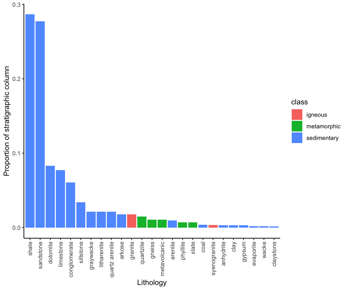
plot of chunk lith_plot
It seems the San Juan Basin is dominated by sedimentary rocks. Perhaps this is not surprising given that we know it is famed for fossils and energy resources! Speaking of these, let’s take a look at the column’s economic attributes:
# Print a summary of economic attributes of the San Juan Basin column
san_juan$econ
## [[1]]
## name type class prop econ_id
## 1 oil reservoir hydrocarbon energy 0.0345 4
## 2 gas reservoir hydrocarbon energy 0.0345 5
## 3 gas indet. hydrocarbon energy 0.4138 8
## 4 oil indet. hydrocarbon energy 0.3103 9
## 5 uranium ore nuclear energy 0.1034 10
## 6 coal coal energy 0.0690 13
## 7 aquifer aquifer water 0.0345 17Here we can see that not only does the San Juan Basin contain coal, oil, and natural gas, but it also has some uranium ore and aquifers. We can also see the number of Paleobiology Database collections linked to the San Juan Basin in our column information:
# Print number of PBDB collections
san_juan$pbdb_collections
## [1] 646To view more information about these fossil data, we need to use a
different rmacrostrat function,
get_fossils:
# Retrieve fossils associated with the San Juan Basin column
sj_fossils <- get_fossils(column_id = 489)
This table contains information about each of the ~650 Paleobiology Database collections associated with the San Juan Basin, including their ages and the number of occurrences they contain. Let’s find out how many fossil occurrences we have in total:
# How many fossil occurrences are associated with the San Juan Basin?
sum(sj_fossils$pbdb_occs)
## [1] 2151So over 2000 fossils are known from this single basin. We can also visualize the temporal distribution of these fossil collections, using the midpoint of their age ranges:
# Add midpoint age for plotting
sj_fossils$m_age <- (sj_fossils$b_age + sj_fossils$t_age) / 2

# Plot of fossil occurrence counts from the San Juan Basin through time
ggplot(sj_fossils, aes(x = m_age)) +
  # Histogram with bars 5 million years wide
  geom_histogram(binwidth = 5, boundary = 0) +
  # Label y-axis
  scale_y_continuous("Number of fossil collections") +
  # Label x-axis and reverse direction
  scale_x_reverse("Time (Ma)", breaks = c(250, 200, 150, 100, 50)) +
  # Theming
  theme_bw() +
  # Add geological timescale
  coord_geo()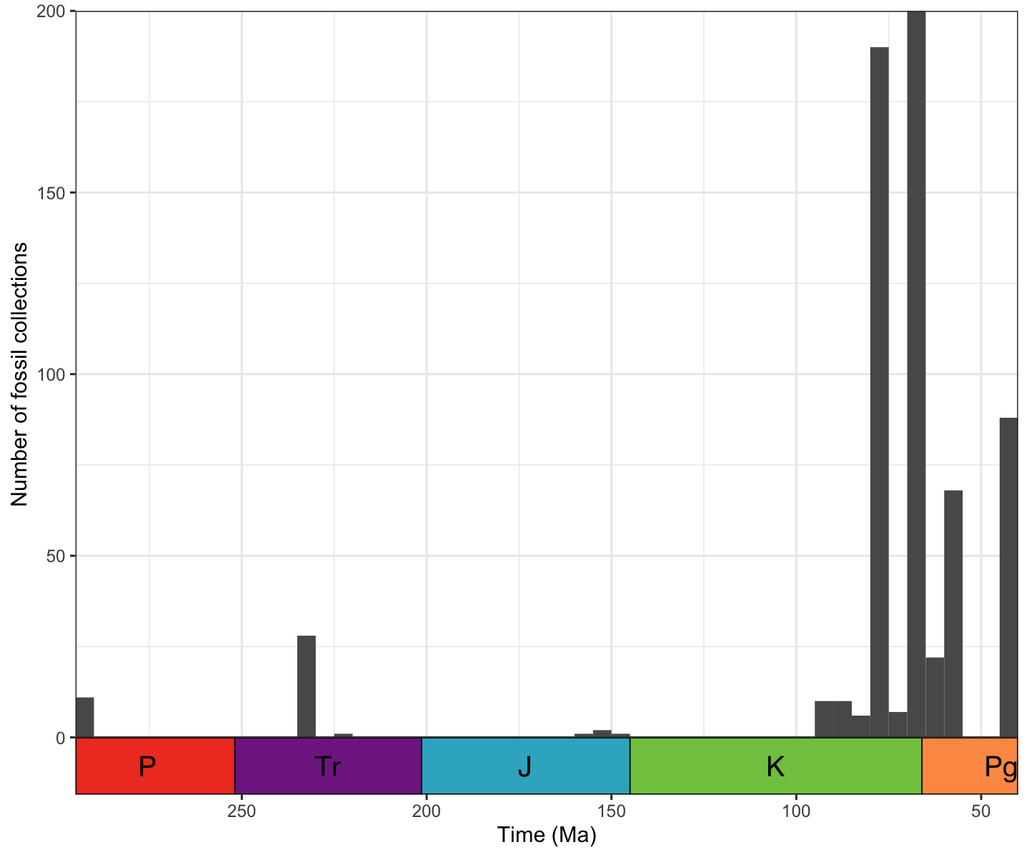
plot of chunk fossil_plot
From this plot, we can see that the San Juan Basin fossils range in age from the Permian to the Paleogene, but we have the highest concentration of fossil collections around the K-Pg boundary. Now that we have explored the data in the Macrostrat database on the San Juan Basin, it is time to plot our stratigraphic column.
Plotting the stratigraphic column
To plot the stratigraphic column, we will need to obtain data for
each lithological unit contained within the San Juan Basin column. We
will do this using another rmacrostrat function,
get_units, and referencing the column_id for
the San Juan Basin. To keep our column plot contained, we will limit it
to geological units which are Cretaceous in age:
# Using the column ID, retrieve the units in the San Juan Basin column
san_juan_units <- get_units(column_id = 489, interval_name = "Cretaceous")
# See the column names and number of rows
colnames(san_juan_units)
## [1] "unit_id" "section_id" "col_id" "project_id"
## [5] "col_area" "unit_name" "strat_name_id" "Mbr"
## [9] "Fm" "Gp" "SGp" "t_age"
## [13] "b_age" "max_thick" "min_thick" "outcrop"
## [17] "pbdb_collections" "pbdb_occurrences" "lith" "environ"
## [21] "econ" "measure" "notes" "color"
## [25] "text_color" "t_int_id" "t_int_name" "t_int_age"
## [29] "t_prop" "units_above" "b_int_id" "b_int_name"
## [33] "b_int_age" "b_prop" "units_below" "strat_name_long"
## [37] "refs" "clat" "clng" "t_plat"
## [41] "t_plng" "b_plat" "b_plng"
nrow(san_juan_units)## [1] 17We now have information for each of the 17 Cretaceous geologic units
contained within the San Juan Basin, including the age of the top and
bottom of each, which is what we will use to plot our stratigraphic
column. To reiterate, the y-axis on our plot is going to be time rather
than height or thickness, so any unconformities present in the column
will be evident. We can start out very simply, by using
geom_rect in ggplot2 to plot a rectangle
corresponding to the age range of each unit in the section.
# Plot stratigraphic column
ggplot(san_juan_units, aes(ymin = b_age, ymax = t_age, xmin = 0, xmax = 1)) +
  # Plot units
  geom_rect(alpha = 0.5, color = "black") +
  # Reverse direction of y-axis
  scale_y_reverse(limits = c(145, 66), n.breaks = 10, name = "Time (Ma)") +
  # Theming
  theme_classic() +
  theme(legend.position = "none",
        axis.line.x = element_blank(),
        axis.title.x = element_blank(),
        axis.text.x = element_blank(),
        axis.ticks.x = element_blank())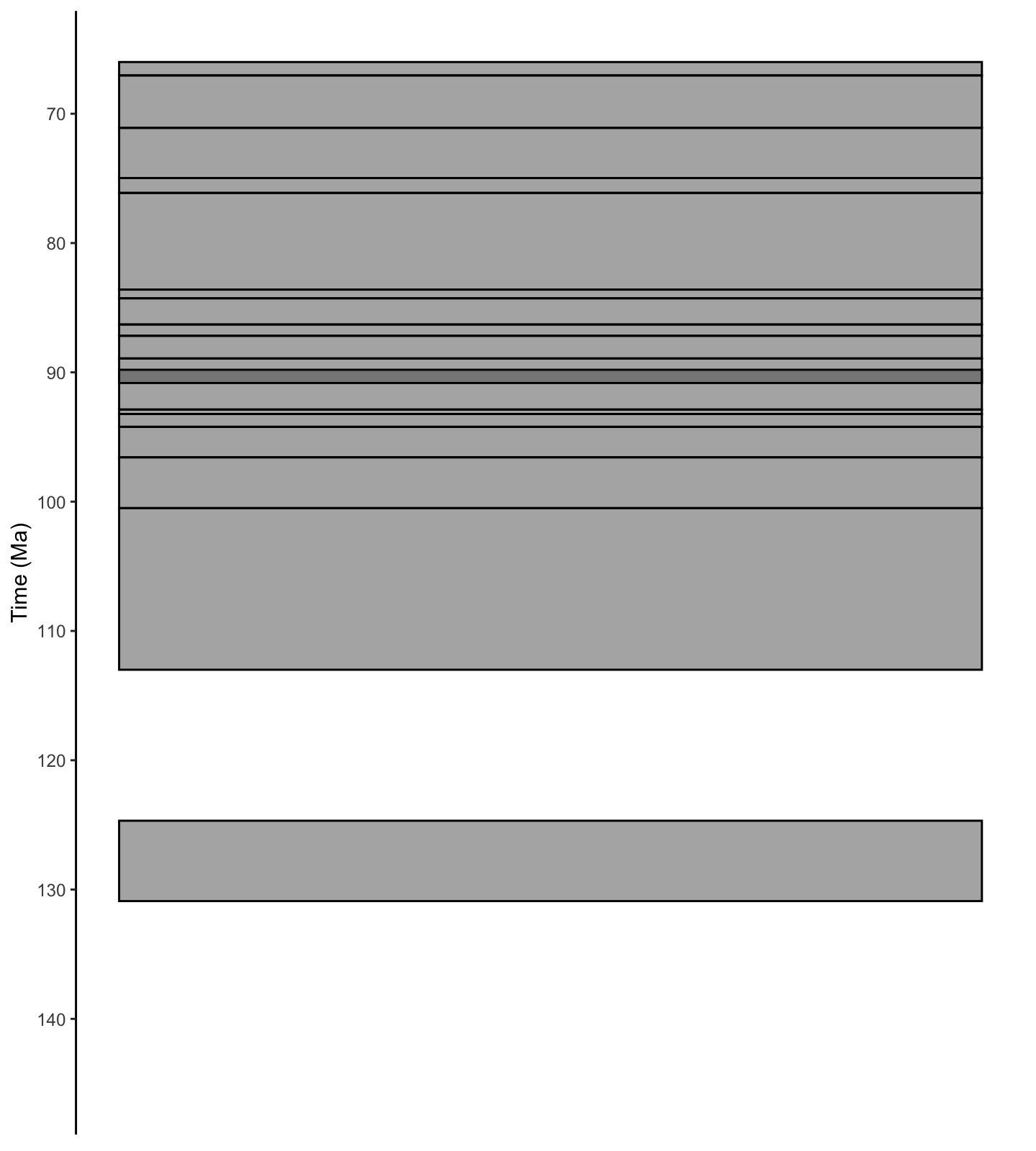
plot of chunk column_a
We can already see something that roughly resembles a stratigraphic column. One thing to notice here is that we seem to have some overlap between our units, resulting in a darker shade of gray. We can take a closer look at this by dodging the units horizontally.
# Plot stratigraphic column
ggplot(san_juan_units, aes(ymin = b_age, ymax = t_age, xmin = 0, xmax = 1)) +
  # Plot units with position dodge
  geom_rect(position = "dodge2", alpha = 0.5, color = "black") +
  # Reverse direction of y-axis
  scale_y_reverse(limits = c(145, 66), n.breaks = 10, name = "Time (Ma)") +
  # Theming
  theme_classic() +
  theme(legend.position = "none",
        axis.line.x = element_blank(),
        axis.title.x = element_blank(),
        axis.text.x = element_blank(),
        axis.ticks.x = element_blank())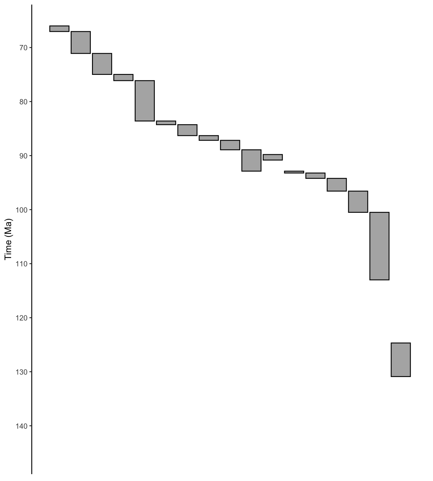
plot of chunk column_b
Indeed, there are two units that overlap with each other: the Gallup Sandstone and the Upper Shale Member of the Mancos Shale. We can make these units plot next to each other by adding columns to our dataframe which define the x-axis values.
# Specify x_min and x_max in dataframe
san_juan_units$x_min <- 0
san_juan_units$x_max <- 1
# Tweak values for overlapping units
san_juan_units$x_max[10] <- 0.5
san_juan_units$x_min[11] <- 0.5

# Plot stratigraphic column
ggplot(san_juan_units, aes(ymin = b_age, ymax = t_age,
                           xmin = x_min, xmax = x_max)) +
  # Plot units
  geom_rect(alpha = 0.5, color = "black") +
  # Reverse direction of y-axis
  scale_y_reverse(limits = c(145, 66), n.breaks = 10, name = "Time (Ma)") +
  # Theming
  theme_classic() +
  theme(legend.position = "none",
        axis.line.x = element_blank(),
        axis.title.x = element_blank(),
        axis.text.x = element_blank(),
        axis.ticks.x = element_blank())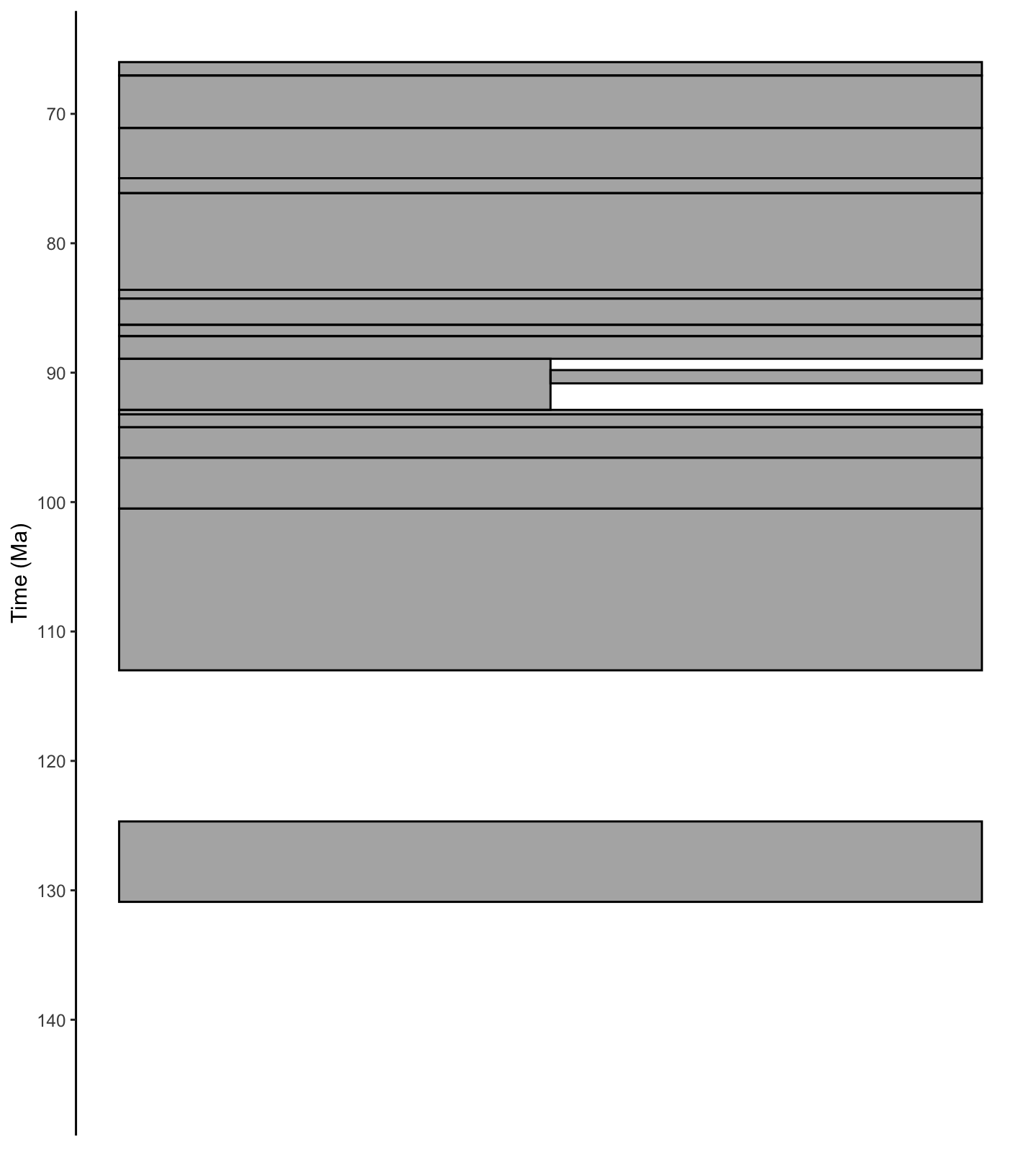
plot of chunk column_c
However, there is a lot we can do to improve the aesthetics of our
plot. For example, the column named color in our dataframe
specifies the hexadecimal color corresponding to the dominant lithology
of the unit. We can use this to color-code the units by lithology.
# Plot stratigraphic column
ggplot(san_juan_units, aes(ymin = b_age, ymax = t_age,
                           xmin = x_min, xmax = x_max)) +
  # Plot units, colored by rock type
  geom_rect(fill = san_juan_units$color, color = "black") +
  # Reverse direction of y-axis
  scale_y_reverse(limits = c(145, 66), n.breaks = 10, name = "Time (Ma)") +
  # Theming
  theme_classic() +
  theme(legend.position = "none",
        axis.line.x = element_blank(),
        axis.title.x = element_blank(),
        axis.text.x = element_blank(),
        axis.ticks.x = element_blank())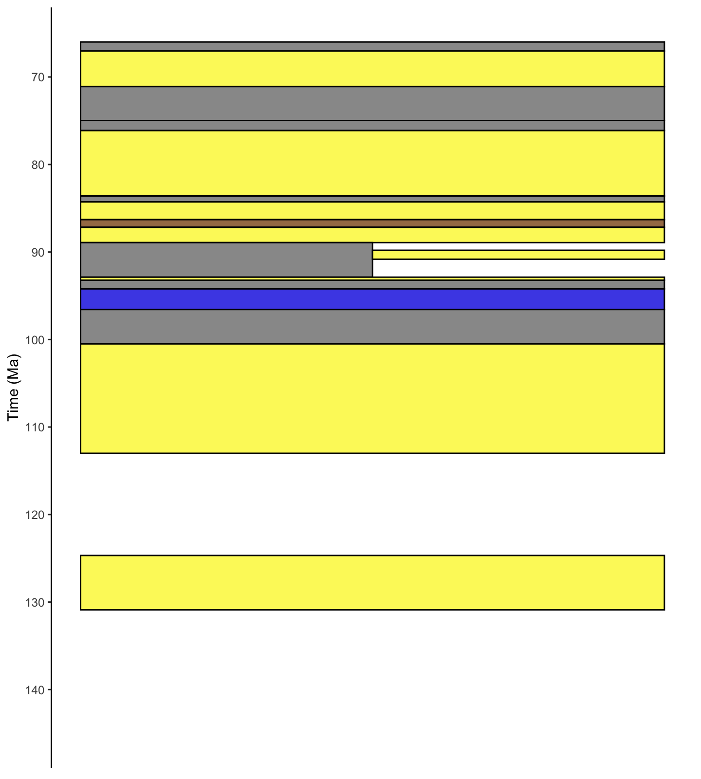
plot of chunk column_d
Great! Now let’s add labels indicating the names of the different units.
# Add midpoint age for plotting
san_juan_units$m_age <- (san_juan_units$b_age + san_juan_units$t_age) / 2

# Plot stratigraphic column
ggplot(san_juan_units, aes(ymin = b_age, ymax = t_age,
                           xmin = x_min, xmax = x_max)) +
  # Plot units, colored by rock type
  geom_rect(fill = san_juan_units$color, color = "black") +
  # Add text labels
  geom_text_repel(aes(x = x_max, y = m_age, label = unit_name),
                  size = 4, hjust = 0, force = 2,
                  min.segment.length = 0, direction = "y",
                  nudge_x = rep_len(x = c(2, 3), length.out = 17)) +
  # Reverse direction of y-axis
  scale_y_reverse(limits = c(145, 66), n.breaks = 10, name = "Time (Ma)") +
  # Theming
  theme_classic() +
  theme(legend.position = "none",
        axis.line.x = element_blank(),
        axis.title.x = element_blank(),
        axis.text.x = element_blank(),
        axis.ticks.x = element_blank())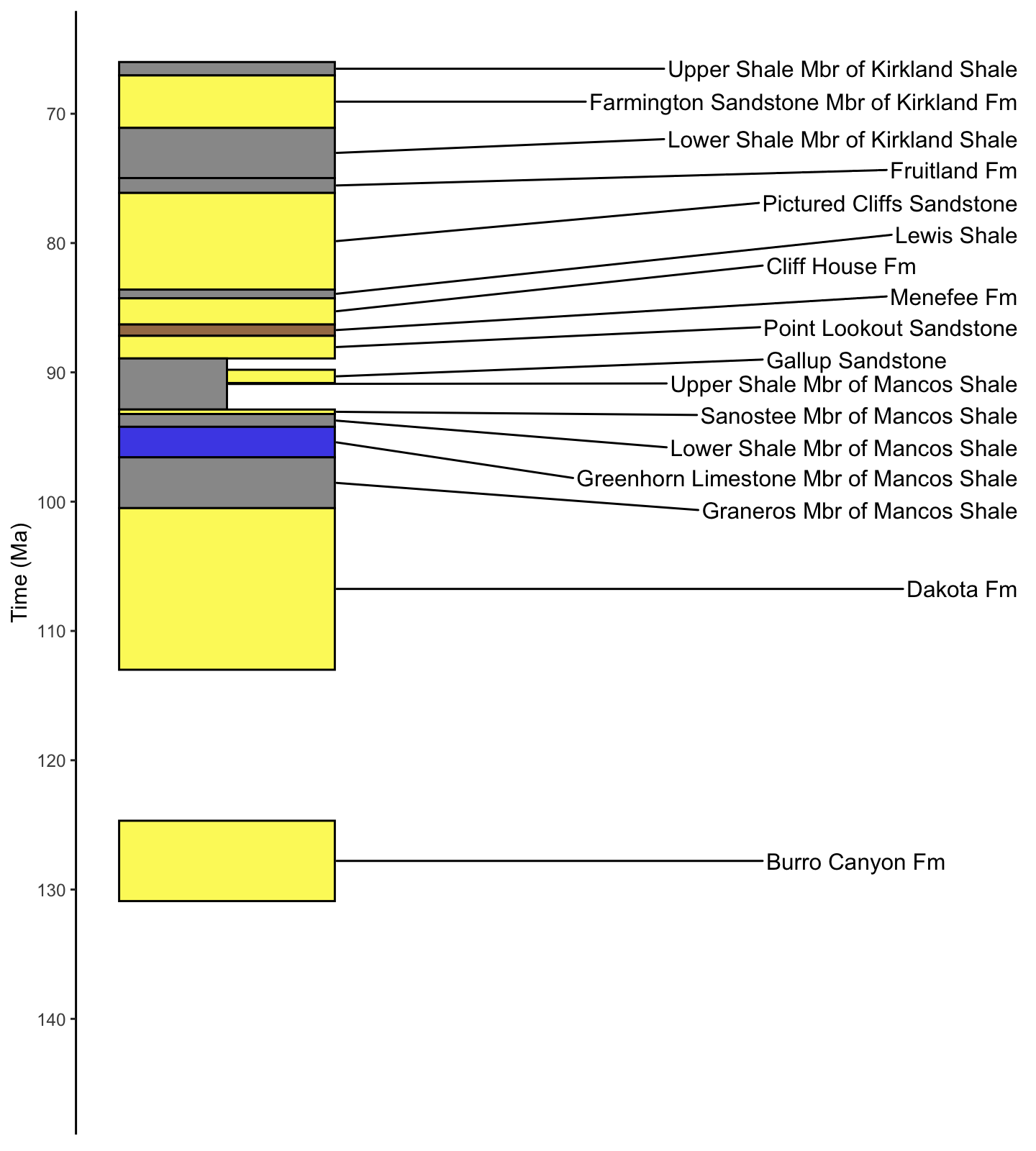
plot of chunk column_e
Oh, we’ve just noticed that some of the unit names seem to have some mistakes and do not match the USGS Geolex. Let’s go ahead and update those names.
# Standardize and correct unit names according to USGS Geolex
san_juan_units$unit_name <- gsub(pattern = "Kirkland",
                                 replacement = "Kirtland",
                                 x = san_juan_units$unit_name)
san_juan_units$unit_name <- gsub(pattern = "Graneros Mbr",
                                 replacement = "Graneros Shale Mbr",
                                 x = san_juan_units$unit_name)
san_juan_units$unit_name <- gsub(pattern = "Sanostee Mbr",
                                 replacement = "Sanastee Sandstone Mbr",
                                 x = san_juan_units$unit_name)
And finally, we can add a column along the y-axis indicating the
different stages of the Cretaceous, using the R package
deeptime:
# Plot stratigraphic column
ggplot(san_juan_units, aes(ymin = b_age, ymax = t_age,
                           xmin = x_min, xmax = x_max)) +
  # Plot units, colored by rock type
  geom_rect(fill = san_juan_units$color, color = "black") +
  # Add text labels
  geom_text_repel(aes(x = x_max, y = m_age, label = unit_name),
                  size = 3.5, hjust = 0, force = 2,
                  min.segment.length = 0, direction = "y",
                  nudge_x = rep_len(x = c(2, 3), length.out = 17)) +
  # Reverse direction of y-axis
  scale_y_reverse(limits = c(145, 66), n.breaks = 10, name = "Time (Ma)") +
  # Theming
  theme_classic() +
  theme(legend.position = "none",
        axis.line.x = element_blank(),
        axis.title.x = element_blank(),
        axis.text.x = element_blank(),
        axis.ticks.x = element_blank()) +
  # Add geological time scale
  coord_geo(pos = "left", dat = list("stages"), rot = 90)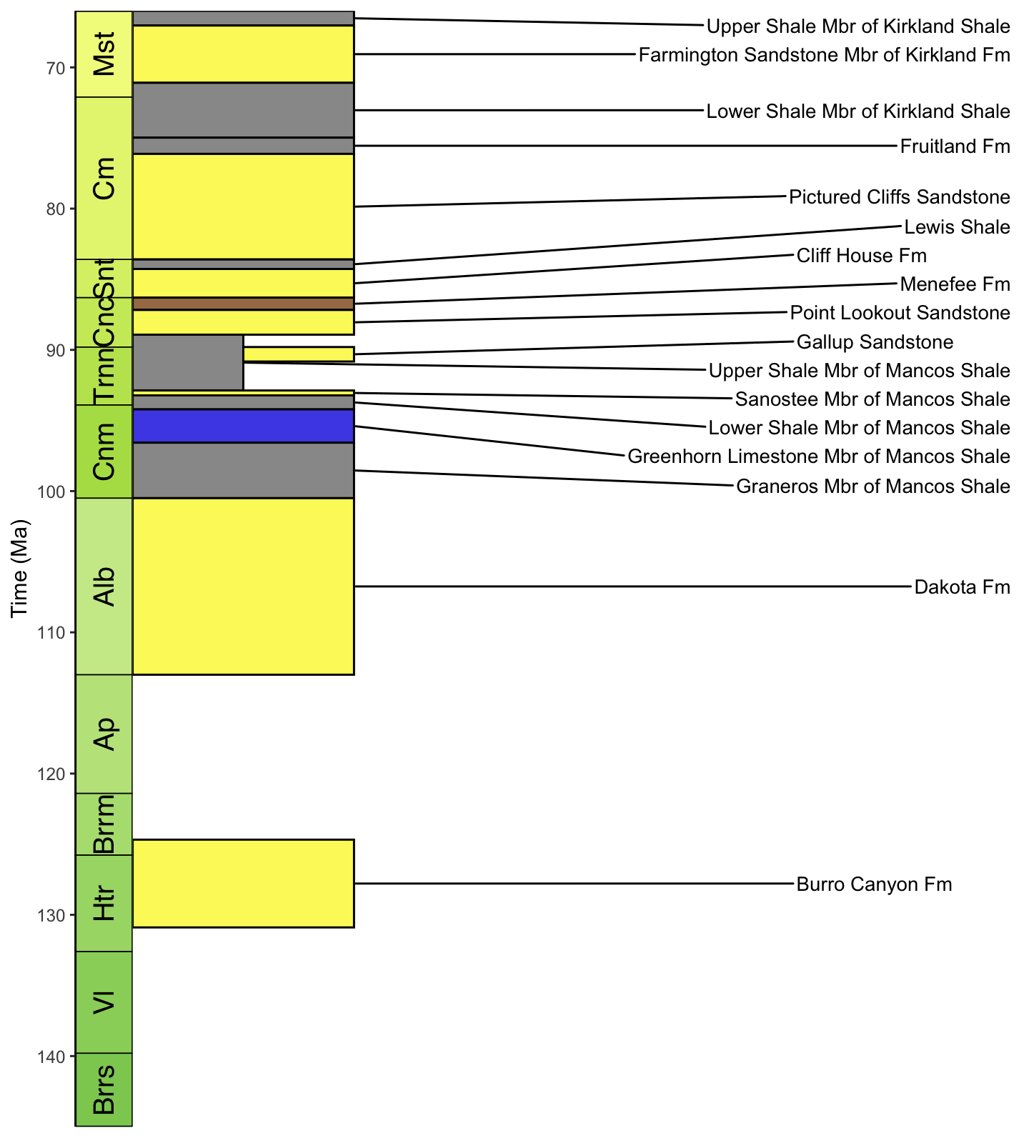
plot of chunk column_f
Hopefully this vignette has shown you the potential uses for
rmacrostrat functions and helped provide a workflow for
your own analyses. If you have any questions about the package or its
functionality, please feel free to join our Palaeoverse Google
group and leave a question; we’ll aim to answer it as soon as
possible!
If you’re interested in learning more about rmacrostrat,
don’t forget to check out our other vignettes! You can see which ones
are available by calling
vignette(package = "rmacrostrat").
References
Gearty, W. 2024. deeptime: Plotting Tools for Anyone Working in Deep Time. R package version 1.1.1, https://CRAN.R-project.org/package=deeptime.
Jones, L.A., Gearty, W., Allen, B.J., Eichenseer, K., Dean, C.D., Galván S., Kouvari, M., Godoy, P.L., Nicholl, C.S.C., Dillon, E.M., Flannery-Sutherland, J.T., Chiarenza, A.A. 2022. palaeoverse: A community-driven R package to support palaeobiological analysis. Methods in Ecology and Evolution, 14(9), 2205–2215. doi: 10.1111/2041-210X.14099.
Wickham, H. 2016. ggplot2: Elegant Graphics for Data Analysis. Springer-Verlag New York.